2024. 4. 17. 00:23ㆍReview/- Network
MLP-Mixer: An all-MLP Architecture for vision
Motivation
The availability of larger datasets coupled with increased computational capacity often leads to a paradigm shift. While CNNs are the go-to model for computer vision. Recently, Vision Transformer (ViT) attained SOTA performance. ViT continues the log-lasting trend of removing hand-crafted visual features and inductive biases from model and relies further on learning from raw data. So authors present MLP-Mixer, an architecture based exclusively on multi-layer perceptrons (MLPs) that are repeatedly applied across either spatial locations or feature channels.
Main Idea
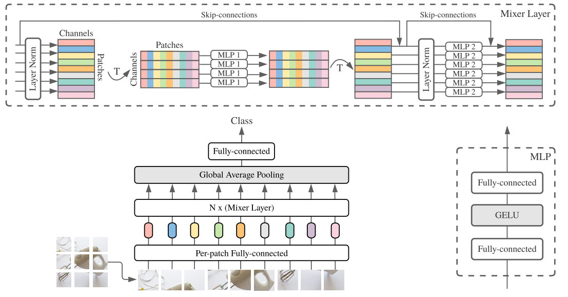
Mixer relies only on basic matrix multiplication routines, changes to data layout (reshape and transpositions), and scalar nonlinearities. Mixer accepts a sequence of linearly projected image patches (tokens) shaped as "patches x channels" table as an input, and maintains this dimensionality. Mixer use two types of MLP layers channel-mixing and token-mixing MLPs. Plain matrix multiplication in MLPs is more simple than convolution as it requires an additional costly reduction to matrix multiplication.
Patch
Mixer takes as input a sequence of $S$ non-overlapping image patches, each one projected to a desired hidden dimension C. If the original input image has resolution ($H,$ $W$), and each patch has resolution ($P$, $P$), then the number of patches is $S=HW/P^2$. All patches are linearly projected with the same project matrix.
Channel-mixing MLP
The channel-mixing MLPs allow communication between different channels. They operate on each token independently and take individual rows of the table as inputs. It can be seen 1x1 convolutions. Channel-mixing MLP acts on rows of $X$.
Token-mixing MLP
The token-mixing MLP allow communication between different spatial locations (tokens). They operate on each channel independently and take individual columns of the table as inputs. It canbe seen single-channel depth-wise convolutions of a full receptive field and parameter sharing. Token-mixing MLP acts on columns of $X^T$. Unlike Vits, Mixer does not use position embeddings because token-mixing MLPs are sensitive.
Mixer Architecture
Modern deep vision architectures consist of layers that mix features (i) at a given spatial location, (ii) between different spatial locations, or both at once. In CNNs 1x1 convolutions perform (i) and larger kernels perform both (i) and (ii). In ViT, self-attention layers allow both (i) and (ii), MLP-blocks perform (i). In MLP-Mixer channel-mixing perform (i) and token-mixing perform (ii). Mixer consists of multiple layers of identical size, and each layer consists of two MLP blocks: token-mixing, channel-mixing MLP. Each MLP block constains two fully-connected layers and a nonlinearity applied in dependently to each row of its input data tensor. ($\sigma$ is GELU)

$D_S$ and $D_C$ are tunable hidden widths in the token-mixing and channel-mixing MLPs. $D_S$, $D_C$ are selected in dependently of the number of input patches. Therefore, the computational complexity of the network is linear (ViT is quadratic). Authors tie parameters of mixing MLPs, it prevents the architecture from growing too fast when increasing the hidden dimension $C$ or sequence length $S$ and leads to significant memory savings.
Aside from the MLP layers, Mixer uses other standard architectural components: sip-connection and layer normalization. Finally Mixer uses a standard classification head with the global average pooling layer followed by a linear classifier.
Experiments
They evalutate the performance MLP-Mixer, pre-trained with meium-to large-scale datasets on mid-sized downstream classification tasks

Downstrema tasks Authors use popular downstream tasks such as ImageNet, ReaL labels, CIFAR-10/100, Oxford-IIIT Pets, Oxford Flowers-102, VTAB-1k.
Pre-training Then follow the standard transfer learning setup: pre-training followed by fine-tuning on the downstream tasks. They pre-train model on two public datasets: ImageNet21k,JFT-300M.
Fine-tuning They also fine-tune at higher resolutions with repect to those used during pre-training. Since they keep the patch resolution fixed, this increases the number of input patches ($S$ to $S'$) and thus requres modifying the shape of Mixer's token-mixing MLPblocks. Eq.(1) is left-multiplied by weight matrix $W_1$ ∈ $R^{D_{s}xS}, For this, tehy increase the hidden layer width from $D_s$ to $D_{s'}$ in proportion to the number of patches and initialize the weight matrix $W'_2$ ∈ $R^{D_{s'}xS'$ with a block-diagonal matrix containing copies of $W_2$ on its diagonal.
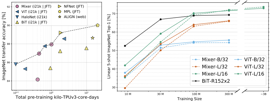
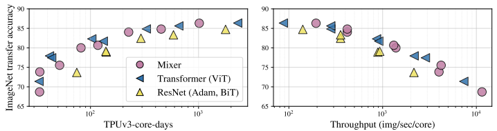
Metrics They evaluate the trade-off between the model's computational cost and quality using (1) Total pre-training time on TPU-v3 accelerators, (2) Throughput in images/sec/core on TPU-v3.
The role of the model scale
They scale the model in two independent ways: (1) Increasing the model size in pre-train, (2) Increasing the input image resolution in fine-tuning
The role of the pre-training dataset size
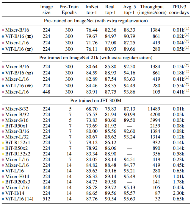
The results presented thus far demonstrate that pre-training on larget datasets significantly improves Mixer's performance. This experiment appears that Mixer benefits from the growing dataset size even more than ViT. One could speculate and explain it again with the difference in inductive bias.
Invariance to input permutations

Authors study the difference between inductive biases of Mixer and CNN architectures by using two kinds of different input transformations. (1) shuffle the order of 16x16 patches and permute pixels within each patch a shared permutation, (2) Permute the pixels globally in the entire image. Mixer is invariant to the order of patches and pixels within the patches. On the other hand, ResNet's strong inductive bias relies on a particular oder of pixels with an image and its performance drops significantly when the patches are permuted.
Concluson
Authors describe a very simple architecture for vision. On the practical size, it may be useful to study the features learned by the model and identify the main difference from those learned by CNNs and Transformers. On the theoretical size, they would like to understand the inductive biases hidden in these various features and eventually their role in generalization.
Reference
[Figure-1~3, Table-1~2]: https://arxiv.org/pdf/2105.01601.pdf
'Review > - Network' 카테고리의 다른 글
| Paper review: SHViT (CVPR 2024) (0) | 2024.05.31 |
|---|---|
| Paper review: Swin Transformer (ICCV 2021) (0) | 2024.04.19 |
| Paper review: ViT (NeurIPS 2021) (0) | 2024.04.15 |
| Paper review: Relational Knowledge Distillation(CVPR 2019) (0) | 2024.04.04 |
| Paper review: CSPNet(CVPR 2020) (0) | 2024.04.03 |