Paper review: DCNv1 (ICCV 2017)

DCNv1: Deformable Convolutional Networks

Motivation

A key challenge in visual recognition is how to accomodate geometric variations or model geometric transformations. In general, there are two ways. The first is to build the training datasets with sufficient desired variations by augmenting the existing data samples like affine transformation. The second is  to use transformation-invariant features and algorithms such as SIFT and sliding window. There are two drawbacks in above ways First the geometric transformation are assumed fixed and known from heuristic manual to augment the data and design the feature and algorighms. Scond, hand crafted design of invaiant features and algorithms could be difficult or infeasible for overly complex transforms. So authors introduce enw modules to enhance the transformation modeling capability of CNNs, namely deformable convolution and deformable RoI pooling.

 

Main Idea

Deformable Convolution

It adds 2D offsets to the regular grid sampling location in the standard convolution. The offsets are learned from the preceding feature maps, via additional convolutional layers.

[Figure-1] Illustration of the sampling locations in 3x3 convolutions

[Figure-2] 3x3 deformable convolution

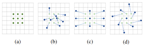
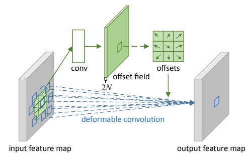
The 2D convolution consist of two steps: 1) sampling using a regular grid $R$ over the input feature map x. 2) summation of smapled values weighted by w. The grid $R$ defines the receptive field size and dilation.

[Eq-1] Calculation of standard convolution

In deformable convolution, the regular grid $R$ is augmented with offsets {$\Delta p_n|n=1,..., N$}, where $N$ = $|R|$.

[Eq-2] Calcuation of deformable convolution

As the offset $\Delta p_n$ is typlically fractional, [Eq-2] is implemented via bilinear interpolation.

[Eq-3] Calcuation of bilinear interpolation

The offsets are obtained by applying a convolution layer over the same input feature map. the convolution kernel is the same spatial resolution and dilation as those of the current convolutional layer. The ouput offset field have the same spatial resolution with the input feature map. The channel dimension 2N corresponds to N 2d offsets.

Deformable RoI Pooling

RoI pooling is used in all region proposal based object detection methods. It convert an input rectangular region of arbirary size in to fixed size features.

[Figure-3] 3x3 deformable RoI pooling

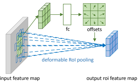
RoI pooling divides the RoI into $k$ x $k$ bins and output a $k$ x $k$ feature map y.

[Eq-4] Calcuation of RoI pooling

where $n_{ij}$ is the number of pixels in the bin. The $(i, j)$-th bin spans $\left \lfloor{i\frac{w}{k}}\right \rfloor$ ≤ $p_x$ < $\left \lceil{(i+1)\frac{w}{k}}\right \rceil$ and $\left \lfloor{j\frac{h}{k}}\right \rfloor$  ≤ $p_y$ < $\left \lceil{(j+1)\frac{h}{k}}\right \rceil$.

[Eq-5] Calcuation of deformable RoI pooling

Also $\Delta p_{ij}$ is fractional, [Eq-5] is implemented by bilinear interpolation.

 

[Figure-3] illustrated how to obtain the offsets. Firstly RoI pooling generates the pooled feature maps. From the maps a fc layer generates the normalized offstet $\Delta \hat{p_ij}$, which are then transformed to the offsets $\Delta p_{ij}$ by element-wise product with the RoI's width and height, as $\Delta p_ij$ = $\gamma \Delta \hat{p_{ij}} ◦(w,h)$. $\gamma$ is pre-defined scalar to modulate the magnitude of the offsets.

 

Experiments

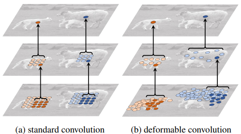
Adaptive receptive field of deformable convolution have more large receptive field than fixed receptive filed of standard convolution. When the deformable convolution ar stacked, the effect of composited deformation is profound.

[Figure-4] Comparison with standard convolution and deformble convolution

[Figure-5] Visualize of sampling locations from deformable convolution

[Figure-6] offset parts in deformable RoI pooling

 

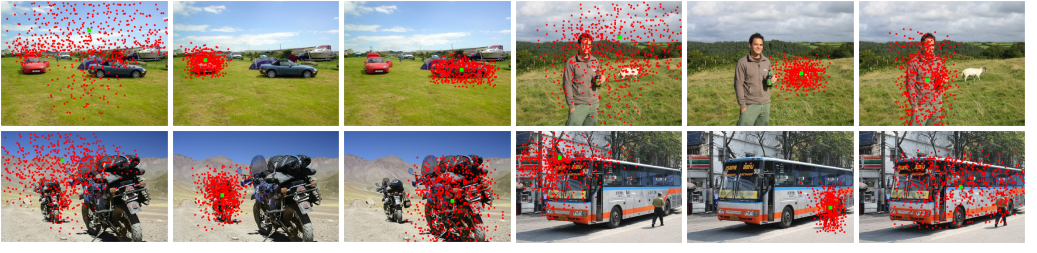
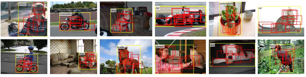
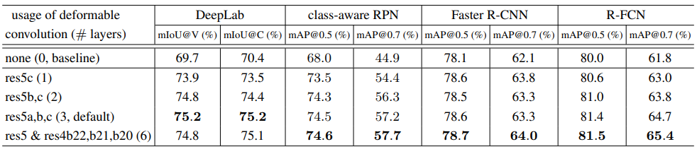
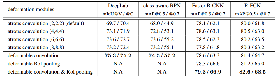
We can check performance of deformable convolution and RoI pooling below table.

[Table-1] Results of using deformable convolution in ResNet-101 on voc 2007 test

[Table-2] Statistics of effective dilation values of deformable convoutional filters

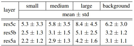
Also we can compare deformable convolution with atrous convolution. Simply we can think deformable convolution is generalized atrous convolution.

[Table-3] Evaluation of deformable modules and atrous convolution

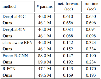
At last we can compare model complexity and runtime comarison of deformable convnets and plain couterparts.

[Table-4] Model complexity and runtime comparison

Conclusion

Authors introduce deformable ConvNets, which is a simple efficient, deep and end-to-end solution to model dense spatial transformations. For the first time they show that it is feasible and effective to learn dense spatial transformation in CNNs.

 

Reference

[Figure-1~6, Eq-1~5, Table-1~4]: https://arxiv.org/pdf/1703.06211